JSON File Configuration

This chapter describes various parameters required for compiling an ONNX model using the DX_COM. It includes input specifications, calibration methods, data preprocessing settings, and optional parameters for advanced compilation schemes.

These parameters are defined in a JSON file, which serves as a blueprint for how the compiler interprets and processes the input model.

---

Parameter Quick Reference

Parameter	Required	Description
inputs	Yes	Model input name and shape: {"name": [1,C,H,W]}
calibration_method	Yes	Calibration method: "ema" or "minmax"
calibration_num	Yes	Number of calibration samples (e.g., 100)
default_loader	Yes	Preprocessing configuration with dataset loading
quantization_device	No	Target device for quantization computation. GPU auto-selected if available
enhanced_scheme	No	DXQ-P0~P5 quantization enhancement for accuracy improvement (DX-COM v2.1.0+)
ppu	No	Object detection post-processing (YOLO models)

For complete examples, see Common Use Cases.

---

Required Parameters

Inputs

Defines the input name and shape of the ONNX model.

Model Input Restrictions

• The batch size must be fixed to 1.
• Only a single input is supported when compiling from a JSON configuration with the dxcom command. For multi-input models, use the dx_com Python module with DataLoader (see Python Wheel Package Usage).
• Input name must exactly match ONNX model definition.

Example

{
  "inputs": {
    "input.1": [1, 3, 512, 512]
  }
}

In this example, "input.1" is the name of the input tensor and its shape is [1, 3, 512, 512], where:

• 1: batch size (must be 1)
• 3: number of channels (e.g., RGB)
• 512 x 512: image height and width

---

Calibration Method

Defines the calibration method used during quantization. It is essential for maintaining model accuracy after compilation by determining appropriate activation ranges.

Available Methods

• ema:
  Uses exponential moving average of activation values.
  Recommended for improved post-quantization accuracy.

• minmax:
  Uses the minimum and maximum activation values to determine quantization range.

Example

{
  "calibration_method": "ema"
}

---

Calibration Number

Defines the number of steps used during calibration. A higher number may improve quantization accuracy by better estimating activation ranges, but may also increase compile time.

To minimize the accuracy degradation, it is recommended to try different values, such as 1, 5, 10, 100, or 1000, and determine the value that yields the best accuracy for your model.

Example

{
  "calibration_num": 100
}

---

Calibration Data Loading

You must provide calibration data using the default_loader parameter, which specifies the dataset location, accepted file types, and preprocessing steps:

{
  "default_loader": {
    "dataset_path": "/datasets/ILSVRC2012",
    "file_extensions": ["jpeg", "png", "jpg", "JPEG"],
    "preprocessings": [
      {"resize": {"width": 224, "height": 224}},
      {"normalize": {"mean": [0.485, 0.456, 0.406], "std": [0.229, 0.224, 0.225]}}
    ]
  }
}

For all available preprocessing operations, see Appendix: Preprocessing Operations Reference.

For Multi-Input Models or Non-Image Data

If you need to compile multi-input models or provide non-image data, use the dx_com Python module with torch DataLoader instead of JSON configuration. See Python Wheel Package Usage.

---

Optional Parameters: Quantization Device

Specifies the device used for quantization during compilation. By default, DX-COM automatically detects available hardware and uses GPU if a CUDA-compatible GPU is available, otherwise falls back to CPU. You can override this behavior by explicitly setting the device.

Available Values

• Not specified (Default): Auto-detect. Uses GPU if available, otherwise CPU.
• "cpu": Force CPU quantization.
• "cuda": Use the default CUDA GPU.
• "cuda:N": Use a specific GPU (e.g., "cuda:0", "cuda:1").

Example

{
  "quantization_device": "cuda:0"
}

Hardware Requirements

• GPU: NVIDIA GPU with CUDA support.
• Framework: PyTorch built with CUDA support (torch.cuda.is_available() must return True).

For practical examples, see Use Case 5: Enhanced Quantization (DXQ).

---

Optional Parameters: Enhanced Quantization Scheme (DXQ)

Version Support

DXQ (enhanced_scheme) is supported in DX-COM v2.1.0 and later.

When quantizing a model, accuracy degradation may occur compared to the original model. To mitigate this, Q-PRO options (DXQ-P0 to DXQ-P5) can be used to enhance quantization performance.

Name	Compilation Speed	Accuracy Improvement
DXQ-P0	Very Fast	Low
DXQ-P1	Fast	Low-Middle
DXQ-P2	Quite Slow	Middle-High
DXQ-P3	Very Slow	High
DXQ-P4	Very Slow	High
DXQ-P5	Very Slow	High

Recommendation

Best Accuracy: DXQ-P3 and DXQ-P4 generally offer better accuracy, so try them first.

GPU Acceleration: DXQ schemes (especially P2-P5) are computationally intensive. Using quantization_device="cuda" can reduce compilation time by 2-5x compared to CPU. See Use Case 5: Enhanced Quantization (DXQ) for examples.

Limitations

Results are not guaranteed to improve accuracy. Results may vary depending on the model and dataset.

DXQ-P0
Uses an alpha value to control the strength of the quantization enhancement.

{
  "enhanced_scheme": {
    "DXQ-P0": {
      "alpha": 0.5
    }
  }
}

DXQ-P1
Enables a simple quantization improvement strategy.

{
  "enhanced_scheme": {
    "DXQ-P1": true
  }
}

DXQ-P2
Uses a more refined strategy with alpha, beta, and cosim_num parameters.

{
  "enhanced_scheme": {
    "DXQ-P2": {
      "alpha": 0.1,
      "beta": 1.0,
      "cosim_num": 2
    }
  }
}

DXQ-P3, DXQ-P4, DXQ-P5
Support the optional num_samples parameter. Recommended value: 1024.

{
  "enhanced_scheme": {
    "DXQ-P3": {
      "num_samples": 1024
    }
  }
}

---

Optional Parameters: PPU Configuration

The Post-Processing Unit (PPU) is a hardware module inside the NPU for accelerating selected post-processing steps in supported object detection models. The ppu configuration section exists to enable this hardware path and provide the parameters required to use it.

In this section, type = 0 and type = 1 still configure PPU hardware paths. type = 2 is different: it does not use the PPU hardware. Instead, it enables an additional CPU-side TopK-based optimization flow for compatible DFL-based YOLO models.

These configurations can automate or optimize the following operations:

• Confidence Filtering (type = 0, type = 1): Removal of detection candidates below a specified threshold through the PPU hardware path.
• Class Prediction (type = 0, type = 1): Execution of Argmax-style class selection per detection through the PPU hardware path.
• TopK Candidate Reduction (type = 2): CPU-side selection of the highest-scoring candidates to reduce the work required in later CPU-side decoding and filtering stages for supported DFL-based YOLO models.

IMPORTANT

NMS (Non-Maximum Suppression) is not supported by the PPU hardware and must still be executed on the host CPU after compilation using the filtered model outputs.

---

Operational Guidelines

Before using the ppu configuration, verify that your model architecture and system requirements align with the following criteria:

Recommended Use Cases (Enable)

• Model Compatibility: Optimized for the YOLO family and similar object detection architectures.
• Hardware Constraints: Highly recommended for edge devices with limited CPU overhead.
• Performance Goals: Necessary for real-time applications requiring high FPS (Frames Per Second).

Non-Supported Scenarios (Disable)

• Classification Models: (e.g., ResNet, MobileNet) These models do not require the filtering logic provided by the PPU.
• Segmentation Models: (e.g., DeepLab, U-Net) These rely on pixel-level mask processing, which is incompatible with PPU logic.
• Custom Architectures: Any model utilizing a detection head that does not align with standard YOLO-style output tensors.

---

Performance Impact

The performance effect depends on the selected PPU type. type = 0 and type = 1 reduce CPU-side detection work through the PPU hardware path, while type = 2 improves CPU-side post-processing efficiency by shrinking the candidate set before the heavier CPU-side DFL-based decoding and later filtering stages.

PPU Mode	Primary Effect	Expected Benefit
Disabled	All post-processing remains on the host CPU	Higher CPU workload
type = 0 / type = 1	The compiled model uses the PPU path for filtering and class prediction	Lower CPU utilization and lower end-to-end latency
type = 2	TopK and the later decoding/filtering stages remain on the host CPU; TopK reduces the number of candidates processed later	Reduced CPU post-processing complexity and improved runtime efficiency

---

Configuration Parameters

Type	Architecture	Supported Models
0	Anchor-Based	YOLOv3, YOLOv4, YOLOv5, YOLOv7
1	Anchor-Free	YOLOX, YOLOv8, YOLOv9, YOLOv10, YOLOv11, YOLOv12
2	DFL-Based Anchor-Free	YOLOv8, YOLOv9, YOLOv10, YOLOv11, YOLOv12 (optional CPU-side TopK optimization path; validated in DX-COM v2.3.0)

---

Type 0: Anchor-Based YOLO Models

{
  "ppu": {
    "type": 0,
    "conf_thres": 0.25,
    "activation": "Sigmoid",
    "num_classes": 80,
    "layer": {
      "Conv_245": {"num_anchors": 3},
      "Conv_294": {"num_anchors": 3},
      "Conv_343": {"num_anchors": 3}
    }
  }
}

Parameters:

• type: Set to 0 for anchor-based models
• conf_thres: Confidence threshold (fixed at compile time)
• num_classes: Number of detection classes
• activation: Typically "Sigmoid"
• layer: Dictionary mapping Conv node names to anchor configurations

---

Type 1: Anchor-Free Models

YOLOX Example:

{
  "ppu": {
    "type": 1,
    "conf_thres": 0.25,
    "num_classes": 80,
    "layer": [
      {"bbox": "output_bbox_1", "obj_conf": "output_obj_1", "cls_conf": "output_cls_1"},
      {"bbox": "output_bbox_2", "obj_conf": "output_obj_2", "cls_conf": "output_cls_2"},
      {"bbox": "output_bbox_3", "obj_conf": "output_obj_3", "cls_conf": "output_cls_3"}
    ]
  }
}

YOLOv8/v9/v10/v11/v12 Example:

{
  "ppu": {
    "type": 1,
    "conf_thres": 0.25,
    "num_classes": 80,
    "layer": [
      {"bbox": "Mul_441", "cls_conf": "Sigmoid_442"}
    ]
  }
}

Parameters:

• type: Set to 1 for the standard anchor-free PPU path
• conf_thres: Confidence threshold (fixed at compile time)
• num_classes: Number of detection classes
• layer: List of layer configurations
  • bbox: Bounding box output layer
  • obj_conf: Object confidence layer
  • cls_conf: Class confidence layer

---

Type 2: DFL-Based Anchor-Free Models (CPU-Side TopK Optimization)

ppu.type = 2 is an optional CPU-side TopK optimization path for compatible DFL-based anchor-free YOLO models. It does not use the PPU hardware. Post-processing still runs on the CPU, and TopK is also performed on the CPU. By reducing the number of candidate boxes that continue into later CPU-side DFL-based decoding and filtering stages, this option reduces post-processing complexity and improves runtime efficiency.

This option is intended for DFL-based YOLO families that expose separate per-scale bbox and cls_conf head nodes. It is an optional CPU-side optimization path in addition to the standard anchor-free PPU configuration. In internal validation for DX-COM v2.3.0, this path was compile-verified with YOLOv8, YOLOv9, YOLOv10, YOLOv11, and YOLOv12 variants using compatible head mappings.

{
  "ppu": {
    "type": 2,
    "topk": 512,
    "num_classes": 80,
    "layer": [
      {"bbox": "bbox_head_p3", "cls_conf": "cls_head_p3"},
      {"bbox": "bbox_head_p4", "cls_conf": "cls_head_p4"},
      {"bbox": "bbox_head_p5", "cls_conf": "cls_head_p5"}
    ]
  }
}

Parameters:

• type: Set to 2 to compile the CPU-side TopK-optimized flow
• topk: Number of candidates kept before later decoding stages
  • If omitted, DX-COM uses the internal default value
  • 512 is a practical starting point for validated YOLO examples
• num_classes: Number of detection classes
• layer: List of per-scale detection head mappings
  • bbox: Final bbox head node name for a detection scale
  • cls_conf: Final class-confidence head node name for the same scale

Use this option only when the model head structure is compatible with this workflow. A DFL-based output is important, but it is not the only requirement. You must also provide correct per-scale bbox and cls_conf node mappings in the JSON configuration.

---

Implementation: Identifying ONNX Node Names

To configure PPU, you need to identify specific node names in your ONNX model:

Step 1. Open your model in Netron to visualize the ONNX graph

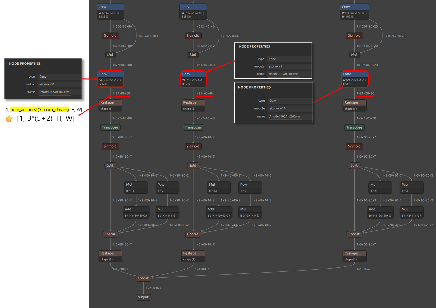
Step 2-1. For Type 0 (Anchor-based YOLO):

• Trace backwards from model outputs to locate detection head Conv layers
• These Conv layers output feature maps with shape [1, num_anchors*(5+num_classes), H, W]
• Example node names in YOLOv7: /model.105/m.0/Conv, /model.105/m.1/Conv, /model.105/m.2/Conv

Step 2-2. For Type 1 (standard anchor-free PPU path, YOLOX example):

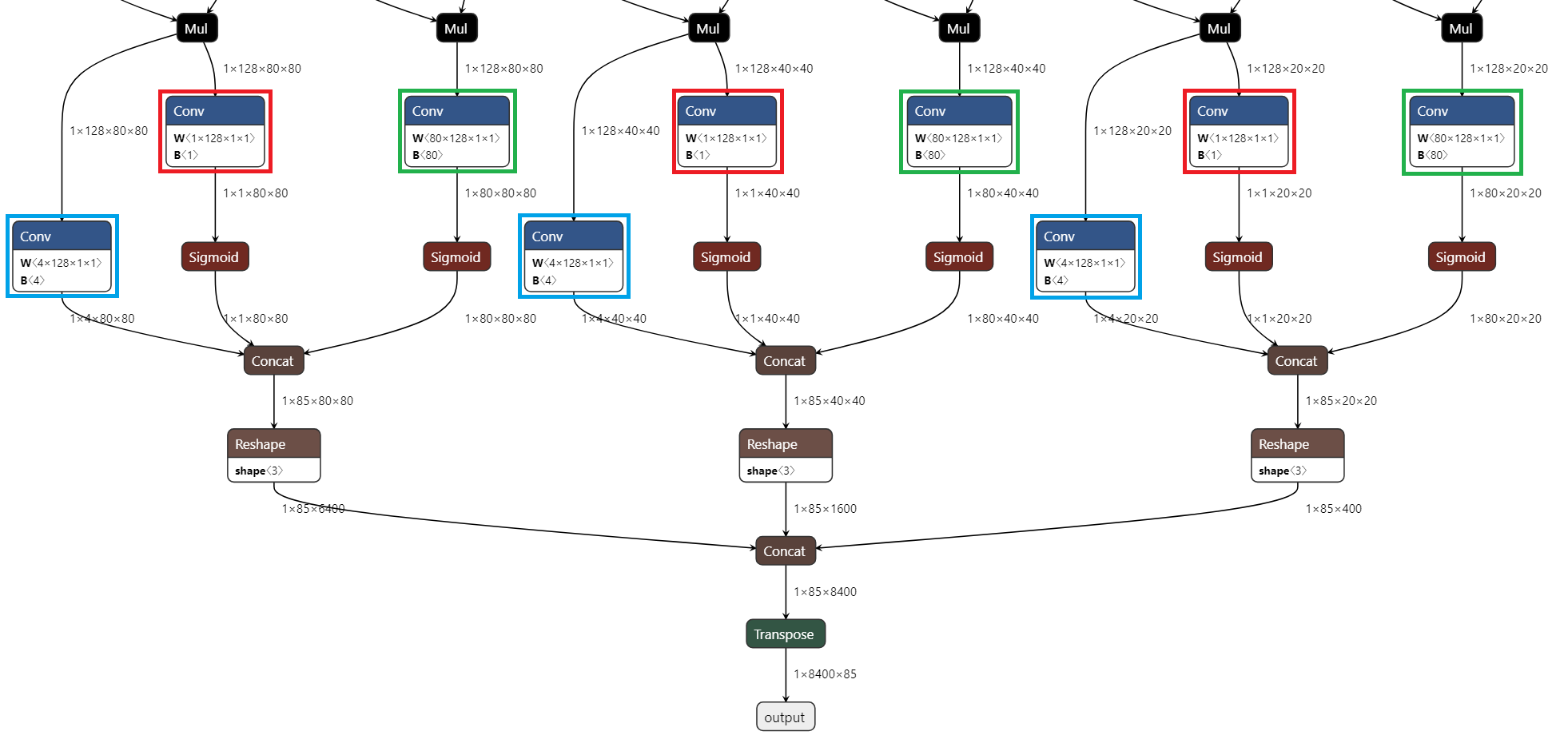
• Find three types of Conv nodes for each detection scale: bbox, obj_conf, cls_conf
• This results in 9 Conv layers total (3 scales × 3 branches)

Step 2-3. For Type 1 (YOLOv8 and later):

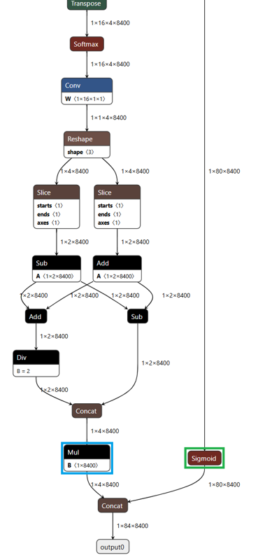
• Trace backwards from the final Concat operation
• Identify bbox (often from Mul or Add) and cls_conf (often from Sigmoid)
• Use the node names that match the layer format required by type = 1

Step 2-4. For Type 2 (CPU-side TopK optimization path):

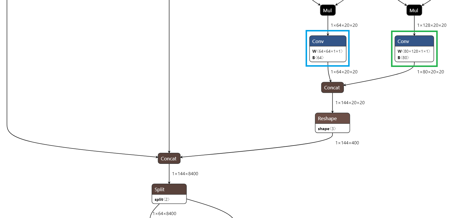
• Inspect the ONNX tail and locate the final per-scale bbox and class head nodes
• Identify three detection scales and pair the matching bbox and cls_conf nodes for each scale
• For validated examples, the correct nodes were the final Conv nodes in the decoupled head branches
• Some models may already include TopK-style operations in the ONNX tail, but you should still map the compatible per-scale bbox / cls_conf nodes for the type = 2 configuration

---

Appendix: Preprocessing Operations Reference

The following preprocessing operations can be applied to input data when using default_loader. These operations help standardize input formats and ensure consistency between calibration and deployment.

Automatic Preprocessing Optimization

To maximize performance, the compiler may automatically integrate specific preprocessing operations directly into the NPU execution graph. This hardware-level integration reduces host CPU load and minimizes data transfer latency.

Optimization depends on input data types and model architecture; therefore, integration is not guaranteed for all operations.

How to Verify and Optimize:

After compilation, inspect the compilation logs for [INFO] - Added nodes: messages. This indicates which operations have been offloaded to the NPU.

1. Identify Integrated Nodes:

Check your log for entries similar to the following: [INFO] - Added nodes: ['Normalize', 'Cast', 'Transpose']

[INFO] - Added nodes: Div(x=255) -> Normalize(mean=[0.485, 0.456, 0.406], std=[0.229, 0.224, 0.225])

2. Update Runtime Code:

If an operation is listed in the "Added nodes" log, it is now handled by the NPU hardware. You must remove these operations from your host-side runtime code to prevent redundant processing and performance degradation.

Status in Log	Action Required	Result
Node Added	Remove from Host Code	Hardware Acceleration Enabled
Node Not Added	Keep in Host Code	Software Preprocessing (CPU)

# If preprocessing is NOT integrated into NPU:
img = img / 255.0
normalized = (img - mean) / std
output = model.run(normalized)

# If preprocessing IS integrated into NPU (log shows "Added nodes"):
output = model.run(img)  # Skip preprocessing - NPU handles it automatically

convertColor

Changes the color channel order of input images.

{"convertColor": {"form": "BGR2RGB"}}

Supported values: RGB2BGR, BGR2RGB, RGB2GRAY, BGR2GRAY, RGB2YCrCb, BGR2YCrCb, RGB2YUV, BGR2YUV, RGB2HSV, BGR2HSV, RGB2LAB, BGR2LAB

resize

Resizes input image to a specified target size.

{"resize": {"mode": "default", "width": 320, "height": 320, "interpolation": "LINEAR"}}

Mode	Supported Interpolation Methods
default (OpenCV)	LINEAR, NEAREST, CUBIC, AREA, LANCZOS4
torchvision (PIL)	BILINEAR, NEAREST, BICUBIC, LANCZOS

centercrop

Crops the central region of the input image.

{"centercrop": {"width": 224, "height": 224}}

transpose

Rearranges tensor dimensions.

{"transpose": {"axis": [0, 2, 3, 1]}}

expandDim

Adds a new dimension at the specified axis.

{"expandDim": {"axis": 0}}

normalize

Normalizes input data by mean and standard deviation. This operation may be integrated into the NPU graph during compilation (see NPU Integration above).

{"normalize": {"mean": [0.485, 0.456, 0.406], "std": [0.229, 0.224, 0.225]}}

mul, add, subtract, div

Arithmetic operations on input data. The subtract and div operations may be integrated into the NPU graph during compilation (see NPU Integration above).

{"mul": {"x": 255}}
{"add": {"x": 128}}
{"subtract": {"x": 127}}
{"div": {"x": 255}}

---

Appendix: Custom Loader (Legacy)

Deprecation Notice

The Custom Loader approach is deprecated. For new projects, use the Python wheel package with torch DataLoader instead, which provides more flexibility and better integration with Python workflows.

For legacy projects that still require Custom Loader, download the Custom Dataloader Guide for detailed instructions.

---